Simulating multivariate effects based on temporal kernel

In the previous example, we showed how to use the toolbox to specify multivariate effects of contrasts between experimental conditions at precise timepoints. You may have noticed that the generated effects look a bit too abrupt temporally to be realistic. That is because, by default, the toolbox generates multivariate effects with the same amplitude at all time points you specified to be present. In real data however, this is not the case. Typically, you would expect decoding to rise not at once but over some time. Similarly, you would not expect the effect to vanish suddenly, but rather to vanish over a period of time.

To simulate more realistic temporal dynamics of multivariate effects, you can specify a temporal kernel that will be convolved with the effects you have specified. In this tutorial, we will illustrate how to do so.

1. Setting up the simulation

Just as in the simulation before, we need to specify a design matrix, the time windows for our effects, as well as the characteristics of our effects (number of channels, number of participants, number of samples per trials…). We will take the same parameters as before.

import numpy as np
import pandas as pd
from scipy.stats import gamma as gamma_dist
import matplotlib.pyplot as plt

# Creating the design matrix of our 2 by two balanced design:
X = np.array([[1, 1, -1, -1] * 40, [1, -1] * 80]).T

# Add descriptors:
cond_names = ["category", "attention"]
X = pd.DataFrame(X, columns=cond_names)  # Add a column for the interaction between category and attention
mapping = {
    "category": {1: "face", -1: "object"},
    "attention": {1: "attended", -1: "unattended"},
}

# Specifying the effects:
effects = [
    {"condition": 'category', "windows": [0.1, 0.2], "effect_size": 0.5}, 
    {"condition": 'attention', "windows": [0.3, 0.4], "effect_size": 0.5}
    ]  # Packaging them in a list to pass to the simulator class

# Data parameters:
n_channels = 32  # EEG system with 32 electrodes
n_subjects = 20  # Recording from 20 subjects
noise_std = 1 / 2  # Variance of the data
ch_cov = None  # Assuming that the data of each sensor are independent
sfreq = 50  # Simulating data at 50Hz
tmin = -0.25
tmax = 1.0

2. Specifying the temporal kernel

To specify mutlivariate effects with more realistic temporal dynamics, we need to define a temporal kernel. This kernel will then be convolved with the time window we have specified for each effect, such that the mutlivariate effects follow these temporal dynamics. To illustrate it, we will use a gamma kernel. A gamma function looks like a Gaussian, except it is skewed towards the right, capturing nicely the typical dynamics of multivariate effect and of ERPs, where we typically see a quick rise followed by a slower decay:

# Generate our kernel:
t = np.arange(0, 1, 1 / sfreq)  # time vector (in seconds)
kernel = gamma_dist(a=2, scale=0.05).pdf(t)
# kernel /= kernel.max()  # Normalize peak to 0.25

# Plot the kernel:
fig, ax = plt.subplots()
ax.plot(t, kernel, label="Gamma (shape=2, scale=0.05)")
ax.legend()
ax.set_title("Gamma Kernel")
ax.set_xlabel("Time (s)")
plt.show()

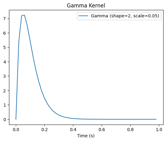
You can play around with the shape and scale parameters to obtain different temporal profiles. I chose these parameters as I thought they look reasonable. Note that here, despite the kernel starting at t = 0, when we convolve it with the data, it will start to rise only from the first sample at which we have an effect and ramp up from there. So don’t try to specify a kernel that starts at the time point you’d want to see your effect, this is taken care of above by specifying the time window for your effect.

4. Simulating the data

The simulation of the data is exactly the same as before, except for the additional kernel parameter:

from multisim import Simulator

sims = Simulator(
    X,  # Design matrix
    effects, # Effects to simulate
    noise_std,  # Observation noise
    n_channels,  # Number of channelss
    n_subjects,  # Number of subjects
    tmin,
    tmax,  # Start and end of epochs
    sfreq,  # Sampling frequency of the data
    ch_cov=ch_cov,  # Spatial covariance of the data
    kern=kernel,  # Temporal kernel
)
epochs = sims.export_to_mne(X=X.copy(), mapping=mapping)

5. Vizualizing the data:

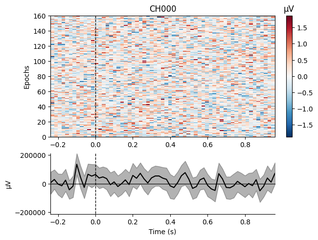
Just as was the case before, we don’t really see much when looking at the activity of a particular channel as we have added effects at the multivariate level. Our kernel doesn’t change anything at that level.

epochs[0].plot_image(picks=[0], scalings=dict(eeg=1));

Not setting metadata

160 matching events found

No baseline correction applied

0 projection items activated

/tmp/ipykernel_3155/238737532.py:1: RuntimeWarning: Cannot find channel coordinates in the supplied Evokeds. Not showing channel locations.
  epochs[0].plot_image(picks=[0], scalings=dict(eeg=1));

6. Decoding analysis

6.1. Within subject analysis:

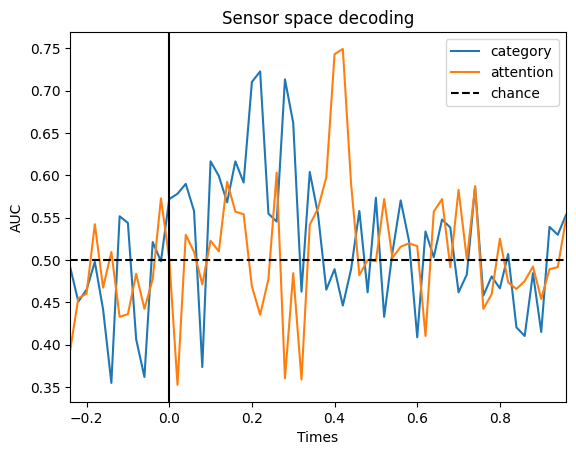
We can try to decode each of the labels of interest (face vs. objects and attended vs. unattended) for a given subject and we will see that these effects are present at the expected time points, but this time following the dynamics defined by our kernel:

import matplotlib.pyplot as plt
import numpy as np
from sklearn.svm import SVC
from sklearn.pipeline import make_pipeline
from sklearn.preprocessing import StandardScaler
from mne.decoding import SlidingEstimator, cross_val_multiscore

# Create the classifier:
clf = make_pipeline(StandardScaler(), SVC())

# Time resolved
time_decod = SlidingEstimator(clf, n_jobs=None, scoring="roc_auc", verbose=True)

# Extract the data:
data = epochs[0].get_data()

# Decode faces vs. objects:
cate_lbl = np.array([mapping["category"][val] for val in X.to_numpy()[:, 0]])
scores_category = np.mean(
    cross_val_multiscore(
        time_decod, data, cate_lbl, cv=5, n_jobs=-1, verbose="WARNING"
    ),
    axis=0,
)

# Decode attended vs. unattended:
att_lbl = np.array([mapping["attention"][val] for val in X.to_numpy()[:, 1]])
scores_attention = np.mean(
    cross_val_multiscore(
        time_decod, data, att_lbl, cv=5, n_jobs=-1, verbose="WARNING"
    ),
    axis=0,
)

# Plot
fig, ax = plt.subplots()
ax.plot(epochs[0].times, scores_category, label="category")
ax.plot(epochs[0].times, scores_attention, label="attention")
ax.axhline(0.5, color="k", linestyle="--", label="chance")
ax.set_xlim([epochs[0].times[0], epochs[0].times[-1]])
ax.set_xlabel("Times")
ax.set_ylabel("AUC")  # Area Under the Curve
ax.legend()
ax.axvline(0.0, color="k", linestyle="-")
ax.set_title("Sensor space decoding")

Text(0.5, 1.0, 'Sensor space decoding')

6.2. Group level analysis

We simulated the data of 20 subjects, so we can investigate the evidence for decoding of the experimental manipulations at the group level. First, we need to perform the decoding on every single subject:

from mne.stats import permutation_cluster_1samp_test, bootstrap_confidence_interval

scores_category = []
scores_attention = []

# Loop through each subject:
for epo in epochs:
    # Extract the data:
    data = epo.get_data()
    # Classification of category
    scores_category.append(
        np.mean(
            cross_val_multiscore(
                time_decod, data, cate_lbl, cv=5, n_jobs=-1, verbose="WARNING"
            ),
            axis=0,
        )
    )
    # Classification of attention:
    scores_attention.append(
        np.mean(
            cross_val_multiscore(
                time_decod, data, att_lbl, cv=5, n_jobs=-1, verbose="WARNING"
            ),
            axis=0,
        )
    )

scores_category = np.array(scores_category)
scores_attention = np.array(scores_attention)

We can then apply a cluster based permutation test across subjects to find out when we have an effect:

# Cluster based permutation test for the category:
T_obs, clusters, cluster_p_values, H0 = permutation_cluster_1samp_test(
    scores_category - 0.5,
    n_permutations=1024,
    tail=1,
    out_type="mask",
    verbose=True,
)
sig_mask_cate = np.zeros(len(epochs[0].times), dtype=bool)
for c, p_val in enumerate(cluster_p_values):
    if p_val < 0.05:
        sig_mask_cate[clusters[c]] = True

# Cluster based permutation test for the attention:
T_obs, clusters, cluster_p_values, H0 = permutation_cluster_1samp_test(
    scores_attention - 0.5,
    n_permutations=1024,
    tail=1,
    out_type="mask",
    verbose=True,
)
sig_mask_att = np.zeros(len(epochs[0].times), dtype=bool)
for c, p_val in enumerate(cluster_p_values):
    if p_val < 0.05:
        sig_mask_att[clusters[c]] = True

Using a threshold of 1.729133

stat_fun(H1): min=-2.8160167131227607 max=14.336126996620614

Running initial clustering …

Found 6 clusters

/opt/hostedtoolcache/Python/3.12.11/x64/lib/python3.12/site-packages/tqdm/auto.py:21: TqdmWarning: IProgress not found. Please update jupyter and ipywidgets. See https://ipywidgets.readthedocs.io/en/stable/user_install.html
  from .autonotebook import tqdm as notebook_tqdm

  0%|          | Permuting : 0/1023 [00:00<?,       ?it/s]

 18%|█▊        | Permuting : 187/1023 [00:00<00:00, 5465.06it/s]

 37%|███▋      | Permuting : 375/1023 [00:00<00:00, 5465.97it/s]

 55%|█████▌    | Permuting : 564/1023 [00:00<00:00, 5472.59it/s]

 74%|███████▍  | Permuting : 758/1023 [00:00<00:00, 5516.96it/s]

 93%|█████████▎| Permuting : 947/1023 [00:00<00:00, 5461.62it/s]

100%|██████████| Permuting : 1023/1023 [00:00<00:00, 5451.50it/s]

Using a threshold of 1.729133

stat_fun(H1): min=-2.1584491283785434 max=12.702962954450564

Running initial clustering …

Found 3 clusters

  0%|          | Permuting : 0/1023 [00:00<?,       ?it/s]

 19%|█▊        | Permuting : 190/1023 [00:00<00:00, 5559.44it/s]

 37%|███▋      | Permuting : 381/1023 [00:00<00:00, 5482.65it/s]

 56%|█████▌    | Permuting : 568/1023 [00:00<00:00, 5435.01it/s]

 74%|███████▍  | Permuting : 760/1023 [00:00<00:00, 5454.64it/s]

 92%|█████████▏| Permuting : 945/1023 [00:00<00:00, 5419.84it/s]

100%|██████████| Permuting : 1023/1023 [00:00<00:00, 5259.25it/s]

100%|██████████| Permuting : 1023/1023 [00:00<00:00, 5267.49it/s]

Based on the input to the simulation, we would expect to see a significantly above chance decoding of face vs. object from 0.1 to 0.2 s, and then of attention from 0.3 to 0.4s. Let’s check whether that is the case:

# Compute the confidence intervals:
ci_low_cate, ci_up_cate = bootstrap_confidence_interval(scores_category)
ci_low_att, ci_up_att = bootstrap_confidence_interval(scores_attention)

fig, ax = plt.subplots()
ax.plot(epochs[0].times, np.mean(scores_category, axis=0), label="category", color="b")
ax.fill_between(epochs[0].times, ci_low_cate, ci_up_cate, alpha=0.3, color="b")
ax.plot(
    epochs[0].times[sig_mask_cate],
    np.ones(np.sum(sig_mask_cate)) * 0.4,
    marker="o",
    linestyle="None",
    color="b",
)

ax.plot(
    epochs[0].times, np.mean(scores_attention, axis=0), label="attention", color="g"
)
ax.fill_between(epochs[0].times, ci_low_att, ci_up_att, alpha=0.3, color="g")
ax.plot(
    epochs[0].times[sig_mask_att],
    np.ones(np.sum(sig_mask_att)) * 0.4,
    marker="o",
    linestyle="None",
    color="g",
)
ax.axhline(0.5, color="k", linestyle="--", label="chance")
ax.set_xlim([epochs[0].times[0], epochs[0].times[-1]])
ax.set_xlabel("Times")
ax.legend()
plt.show()

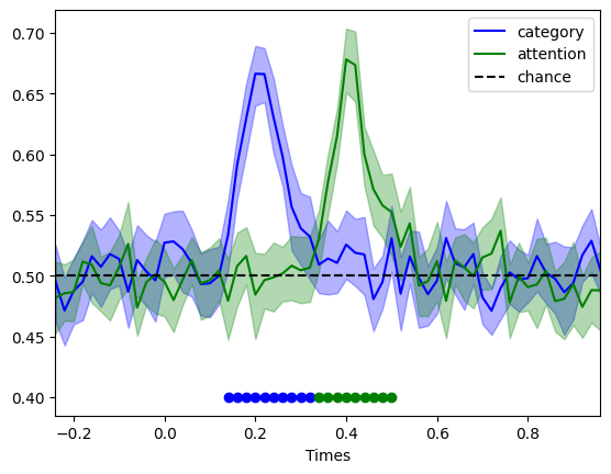
These results align with what we would expect. However, you probably noticed that this time, the effect don’t seem to be restricted to the time points we have specified. That’s to be expected. The gamma kernel are convolved with the time windows of our effects, so the effects gets protruded in time. If you want to avoid this, you should specify your effect as a single point in time (one sample) which when convolved with a temporally extended kernel will become protruded in time. You can then play around with the spread of your kernel to control the duration of the effect. So when using a kernel, it is a bit less straight forward to specify clear time points for your effects.

In the next tutorial, we will show how to specify between subject noise, to make the data even more realistic.