import os
import numpy as np
import pandas as pd
import arviz as az
import matplotlib
import matplotlib.pyplot as plt
import matplotlib.colors as mcolors
from scipy.special import expit
from IPython.display import Markdown, display

from stabst.MarkovDecisionProcess import MDP
from stabst.TaskConfig import LimitedEnergyTask

A4_inches = [8.27-0.5,11.69-0.5]

def make_grid(dv_min, dv_max, pref_min, pref_max):
    """
    Makes a 2D grid reflecting the limits of our modelled variables (preferences and DV)
    Parameters
    ----------
    dv_min : _type_
        _description_
    dv_max : _type_
        _description_
    pref_min : _type_
        _description_
    pref_max : _type_
        _description_

    Returns
    -------
    _type_
        _description_
    """
    x1_grid = np.linspace(start=dv_min, stop=dv_max, num=300)
    x2_grid = np.linspace(start=pref_min, stop=pref_max, num=300)
    x1_mesh, x2_mesh = np.meshgrid(x1_grid, x2_grid)
    x_grid = np.stack(arrays=[x1_mesh.flatten(), x2_mesh.flatten()], axis=1)
    return x1_grid, x2_grid, x_grid

def truncate_colormap(cmap, min_val=0.0, max_val=1.0, n=256):
    """Slice a colormap to the sub-range [min_val, max_val]."""
    colors = cmap(np.linspace(min_val, max_val, n))
    return mcolors.LinearSegmentedColormap.from_list(
        f"{cmap.name}_trunc({min_val:.2f},{max_val:.2f})", colors
    )

def predict_responses(dv, pref, idata):
    """_summary_

    Parameters
    ----------
    dv : _type_
        _description_
    pref : _type_
        _description_
    beta_plan : _type_
        _description_
    beta_interaction : _type_
        _description_
    """
    # Compute the preferences entropy:
    p_pref = expit(pref)
    entropy = -p_pref * np.log(p_pref) - (1-p_pref) * np.log(1 - p_pref)
    # Extract the betas:
    b_plan = idata.posterior["beta_planning"].mean().data
    b_interaction = idata.posterior["beta_interaction"].mean().data
    return expit(b_plan * dv + pref + b_interaction * dv * entropy)
In [1]:
In [2]:
# Load & Prepare the data:
beh_data = pd.read_csv('./data/raw_data/all_participants_data.csv')
# ===================================================================
# Data preprocessing:
# Remove nans:
beh_data = beh_data.dropna()
# Remove timeout:
beh_data = beh_data[beh_data["timeout"] == 0]
# Flip responses: 1 = accept:
beh_data["response"] = (beh_data["response"] == 0).astype(int)
# Make trial 1 based
beh_data["trial"] = beh_data["trial"] + 1
# Generate future cost based on the transitions:
transitions_costs = {
    0: [1, 1],
    1: [2, 1],
    2: [1, 2],
    3: [2, 2]
}
beh_data["fc"] = [transitions_costs[row["transition"]][1] for _, row in beh_data.iterrows()]

# ===================================================================
# Task MDP:
# Create the task and its parameters (transition probability, reward...):
task = LimitedEnergyTask(O=[1, 2, 3, 4], p_offer=[1/4] * 4)
task.build()

# Create full MDP and compute solution for later reference:
gamma = 1
task_mdp = MDP(task.states, task.tp, task.r, gamma, s2i=task.s2i)
V_full, Q_full = task_mdp.backward_induction()

# Add DV to the data frame:
dv = Q_full[:, 1] - Q_full[:, 0]
# Loop through each trial to set DV:
dv_trials = []
for trial_i, trial in beh_data.iterrows():
    e, o, cc, t = trial.energy, trial.reward, trial.energy_cost, trial.trial
    fc = transitions_costs[trial.transition][1]
    dv_trials.append(dv[task.s2i[(e, o, cc, fc, t)]])
beh_data['dv'] = dv_trials
In [3]:
# Load all models:
# Fitting the models:
traces = {}
# ===================================================================
# Preference model:
if os.path.exists("./data/bids/limited_energy/derivatives/models/preferences_model_trace.nc"):
    idata = az.from_netcdf("./data/bids/limited_energy/derivatives/models/preferences_model_trace.nc")
    traces['Preference'] = idata
else:
    raise Exception("You must run index.ipynb first!")

# ===================================================================
# Hybrid model from Ott's
if os.path.exists("./data/bids/limited_energy/derivatives/models/hybrid_model_trace.nc"):
    idata = az.from_netcdf("./data/bids/limited_energy/derivatives/models/hybrid_model_trace.nc")
    traces['Context'] = idata
else:
    raise Exception("You must run index.ipynb first!")

# ===================================================================
# Marginal action distribution model:
if os.path.exists("./data/bids/limited_energy/derivatives/models/action_prior_model_trace.nc"):
    idata = az.from_netcdf("./data/bids/limited_energy/derivatives/models/action_prior_model_trace.nc")
    traces['Frequency prior'] = idata
else:
    raise Exception("You must run index.ipynb first!")

# ===================================================================
# Pure planning model
if os.path.exists("./data/bids/limited_energy/derivatives/models/planning_model_trace.nc"):
    idata = az.from_netcdf("./data/bids/limited_energy/derivatives/models/planning_model_trace.nc")
    traces['Planning'] = idata
else:
    raise Exception("You must run index.ipynb first!")

model_comparison = az.compare(traces)
/home/alex-lepauvre/miniforge3/envs/pymc_env/lib/python3.14/site-packages/arviz/stats/stats.py:782: UserWarning: Estimated shape parameter of Pareto distribution is greater than 0.70 for one or more samples. You should consider using a more robust model, this is because importance sampling is less likely to work well if the marginal posterior and LOO posterior are very different. This is more likely to happen with a non-robust model and highly influential observations.
warnings.warn(
/home/alex-lepauvre/miniforge3/envs/pymc_env/lib/python3.14/site-packages/arviz/stats/stats.py:782: UserWarning: Estimated shape parameter of Pareto distribution is greater than 0.70 for one or more samples. You should consider using a more robust model, this is because importance sampling is less likely to work well if the marginal posterior and LOO posterior are very different. This is more likely to happen with a non-robust model and highly influential observations.
warnings.warn(Figures
In [4]:
# Extract relevant variables from preference model:
beh_data['preference_score'] = np.mean(traces['Preference'].posterior["preference"], axis=(0, 1)).to_numpy()
In [5]:
fig, ax = plt.subplot_mosaic("A;B", figsize=[A4_inches[0], 1*A4_inches[1]], sharex=True, sharey=True)
cmap = matplotlib.colormaps.get_cmap('Set3')

# ================================================================
# fig-3A: Plot the interaction between preferences and decision values:
x1_grid, x2_grid, x_grid = make_grid(beh_data['dv'].min(), beh_data['dv'].max(), beh_data['preference_score'].min(), beh_data['preference_score'].max())

# =================================
# Plot the predicted response probability in the background:
cmap_background = truncate_colormap(plt.get_cmap("RdYlBu_r"),  min_val=0.25, max_val=0.75)
# Create grid:
grid_df = pd.DataFrame(x_grid, columns=["dv", "pref"])
# Simulate responses across the grid:
grid_df["p"] = predict_responses(grid_df["dv"], grid_df["pref"], traces["Preference"])
p_grid = grid_df.pivot(index="pref", columns="dv", values="p").to_numpy()
# Plot contours:
cs = ax["B"].contourf(x1_grid, x2_grid, p_grid, cmap=cmap_background)
ax["B"].clabel(cs, fontsize=10, colors='k')
ax["B"].axvline(0, linestyle=":", color="grey")
ax["B"].axhline(0, linestyle=":", color="grey")
ax["B"].text(-0.05, 1.05, "B", transform=ax["B"].transAxes,
              fontsize=16, fontweight='bold', va='top', ha='right'
              )
ax["B"].spines[['right', 'top']].set_visible(False)
ax["B"].set_xlabel("DV")
ax["B"].set_ylabel("Preference score")

# =================================
# Plot responses as a function of DV and pref:
# Get trials where pref and DV are opposed:
# mismatch accept
mismatch_accept = beh_data[(np.sign(beh_data['dv']) != np.sign(beh_data['preference_score'])) & (beh_data['response'] == 1)]
# mismatch reject
mismatch_reject= beh_data[(np.sign(beh_data['dv']) != np.sign(beh_data['preference_score'])) & (beh_data['response'] == 0)]
# Get the rest:
matched = beh_data[(np.sign(beh_data['dv']) == np.sign(beh_data['preference_score']))]
# Plot each mismatch
ax["A"].scatter(matched['dv'], matched['preference_score'],
                color="grey", marker='o', alpha=0.1,
                label=f'sgn(DV)=sgn(Preferences)')
ax["A"].scatter(mismatch_reject['dv'], mismatch_reject['preference_score'],
                color=cmap(1), edgecolors='black', linewidths=0.5, s=50,
                label=f'Reject (N={mismatch_reject.shape[0]})', marker='h', alpha=0.5)
ax["A"].scatter(mismatch_accept['dv'], mismatch_accept['preference_score'],
                color=cmap(0), edgecolors='black', linewidths=0.5, s=50,
                label=f'Accept (N={mismatch_accept.shape[0]})', marker='v', alpha=0.5)
# Decoration:
ax["A"].set_ylabel("Preference score")
ax["A"].text(-0.05, 1.05, "A", transform=ax["A"].transAxes,
              fontsize=16, fontweight='bold', va='top', ha='right'
              )
ax["A"].axvline(0, linestyle=":", color="grey")
ax["A"].axhline(0, linestyle=":", color="grey")
ax["A"].spines[['right', 'top']].set_visible(False)
ax["A"].legend(frameon=False);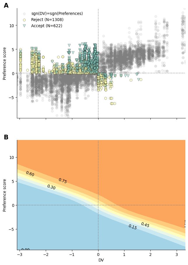
Tables
In [6]:
# Print the model comparison:
display(Markdown(model_comparison[[ "elpd_loo", "p_loo", "elpd_diff", "se", "dse"]].to_markdown()))| elpd_loo | p_loo | elpd_diff | se | dse | |
|---|---|---|---|---|---|
| Preference | -1492.49 | 256.526 | 0 | 48.7651 | 0 |
| Context | -1656.69 | 159.175 | 164.209 | 52.4615 | 19.671 |
| Frequency prior | -2073.38 | 77.0896 | 580.889 | 55.5712 | 35.9363 |
| Planning | -2078.46 | 68.3847 | 585.976 | 55.58 | 36.1456 |
In [7]:
# Print the table as a markdown:
stats_summary = az.summary(traces['Preference'], var_names=["beta_planning", "beta_pref", "beta_interaction"], hdi_prob=0.95)
# Creat the row names:
row_names = ["$\\beta_{plan}$",
             "$\\beta_{O=1}$", "$\\beta_{O=2}$", "$\\beta_{O=3}$", "$\\beta_{O=4}$",
             "$\\beta_{CC=1}$", "$\\beta_{CC=2}$", "$\\beta_{FC=1}$", "$\\beta_{FC=1}$",
             "$\\beta_{E=0}$", "$\\beta_{E=1}$", "$\\beta_{E=2}$", "$\\beta_{E=3}$", "$\\beta_{E=4}$", "$\\beta_{E=5}$", "$\\beta_{E=6}$",
             "$\\beta_{interaction}$"]
stats_summary.index = row_names
display(Markdown(stats_summary[[ "mean", "sd", "hdi_2.5%", "hdi_97.5%" ]].to_markdown()))| mean | sd | hdi_2.5% | hdi_97.5% | |
|---|---|---|---|---|
| \(\beta_{plan}\) | 2.072 | 0.242 | 1.614 | 2.573 |
| \(\beta_{O=1}\) | -2.374 | 0.971 | -4.232 | -0.426 |
| \(\beta_{O=2}\) | -1.625 | 0.938 | -3.535 | 0.092 |
| \(\beta_{O=3}\) | 1.627 | 0.945 | -0.22 | 3.453 |
| \(\beta_{O=4}\) | 2.923 | 0.976 | 1.054 | 4.842 |
| \(\beta_{CC=1}\) | 0.765 | 1.161 | -1.488 | 3.105 |
| \(\beta_{CC=2}\) | -0.127 | 1.165 | -2.482 | 2.144 |
| \(\beta_{FC=1}\) | 0.457 | 1.149 | -1.86 | 2.557 |
| \(\beta_{FC=1}\) | 0.21 | 1.149 | -2.051 | 2.359 |
| \(\beta_{E=0}\) | -4.438 | 0.935 | -6.247 | -2.627 |
| \(\beta_{E=1}\) | -0.48 | 0.781 | -1.994 | 1.076 |
| \(\beta_{E=2}\) | -0.02 | 0.75 | -1.473 | 1.492 |
| \(\beta_{E=3}\) | 0.203 | 0.748 | -1.228 | 1.688 |
| \(\beta_{E=4}\) | 0.3 | 0.758 | -1.186 | 1.799 |
| \(\beta_{E=5}\) | 0.793 | 0.769 | -0.602 | 2.44 |
| \(\beta_{E=6}\) | 4.195 | 0.962 | 2.363 | 6.132 |
| \(\beta_{interaction}\) | 1.306 | 0.508 | 0.258 | 2.256 |