
Probablities and probability distribution#
In the previous section, we mentioned a couple of terms and thought about how to answer a simple question based on some common-sense ideas. While this kind of worked and we were able to get a sense of whether or not our coin is biased, we also couldn’t really know for sure if our reasoning made sense, and ultimately our answer was based on gut-feeling. We can rely on mathematics to do better and get the best possible answer based on How confident we are that our coin isn’t biased based on the results of our experiment or put differently How probable is it that our coin isn’t biased, given the reuslts of our experiment?
Definitions:#
To be able to do that, we need to define a couple of terms we use, and provide some mathematical notation to be able to do some math with them.
Probability: the likelihood of the occurence of a particular event out of all possible events. Our question of whether or coin is fair can be rephrased as “Is the probability of getting head 0.5?”. As there are only two possible outcomes for a coin toss (head or tail), if we have 50% chances of getting head, then we have 50% chances of getting tail and therefore our coin is balanced. The probability of a particular event is written like so:
Which reads: The probability of a particular event occuring is the number of time that particular event occurs divided by the total number of possible events. In probability theory, each of the terms used in the definition of a probability also has a precise definition:
Event: a specific outcome of an experiment. In the case of a coin toss, this is either getting head or tail. But say we want to run another experiment in which we draw a card in a 52 cards deck at random, drawing a king of spade would also be an event for example.
Sample space: set of all possible outcomes of the experiment. In our coin toss example, the sample space is basically head and tail, as these are the only two possible outcomes from throwing a coin. Similarly, if we draw a card from a deck, the sample space is basically all the cards in the deck. And so in the case of a coin toss, the total number of possible outcome in the sample space is 2, but in an experiment where we draw a card, it’s 52.
Number of favorable outcomes for event A: how often does the event occurs out of all the possible outcomes. This is basically the quantity that defines the probability of that particular event.
So in the case of our coin toss example, head is an event and tail is another. If the coin is balanced, we have:
And
We could also have:
In which case our coin isn’t balanced, because head is more likely than tail. This brings us to an important properties that all probabilities have:
This means that when we sum all the probability of each possible event, we always get 1. This makes sense: when we throw a coin, something will always happen, either it lands on head or on tail. There is no scenario in which we toss a coin and the coin doesn’t land on anything. You could argue that the coin could land on the side. Fair, that is a possible outcome, albeit not very likely. But that’s fine with probability theory, we just have to say that when we throw a coin, the sample space cointains head, tail and side. Each should have a probability. But I would argue that tail is really unlikely (never saw it myself, and I tossed a few coins in my days), so we can probably say something like:
\(P(Side)\) is so unlikely that we can ignore it. And so because the sum of the probability of all events in the sample space should be 1 and that we have only two outcomes, then we can say the following:
So
In the case of a coin toss, if we know the probability of one event, we know the probability of the other.
Probability have another important property:
Which means that for any event A, it’s probability is minimally 0 (it can’t happen and will never happen) and maximally 1 (it will always happen). This makes sense in the case of a coin toss: we can’t get two times head when we toss the coin once, we can at most always get head when we throw a coin.
Of course probability theory is not only about tossing coins. We can apply the same definitions we have given above to any random things. For example, if you have a 52 cards deck and you pick a card at random. In this case, picking up a particular card is a specific event, and your sample space is 52, because you have 52 different cards. For example, the probability of picking a King of Spade is described as:
And of picking up a jack of heart:
The same properties described above: the probability of each event is between 0 and 1, and the sum of the probability of all events is 1.
True vs. Observed Probabilities:#
Our question is: Is our coin biased or not. But that is basically the same as asking: Is the probability of obtaining head 0.5?. That’s because if we consider that there are only two possible outcomes to throwing a coin (head or tail), then if:
then
So we have:
In other words, if the probability of getting head is 0.5, so is the probability to get tail and our coin is balanced.
What we want to know is what is the True probability of head. And as we saw in the previous page, we can run an experiment (toss the coin a bunch of times) to try and estimate what that True probability might be to answer our question. In our experiment, we compute a so-called Empirical Probability. There is some uncertainty in the result of our experiment, because the Empirical Probability of getting head changed when we repeated the experiment.
The True probability of an event is typically written as \(P(A)\), while the Empirical probability is depicted as \(\hat{P}(E)\), to make the distinction between the two.
Mathetmatical functions as probability distribution#
In the above examples, we can write the probability of each event one by one: \(P(A=Head)=0.5, P(A=Tail)=0.5\), or \(P(A=King of Spade)=1/52, P(A=King of Heart)=1/52...\)
That is of course a bit cumbersome, and already for the probability of each event when pulling a card from the deck, I got too lazy to write all options. The field of probability theory aims at finding compact and easy formulae to precisely describe the probability of each event in a particular sample space (i.e. the probability of any possible outcome of a given experiment). These are mathematical function that describe the probability of any possible outcome of an experiment, and this kind of functions are called:
Probability distributions: a function that assigns a probability to each possible outcome in a sample space, representing the likelihood of each outcome occurring. It describes how probabilities are distributed over the set of possible outcomes, ensuring that all probabilities are non-negative and that their total sums to one.
These formulae aim to be general enough, so that for any system that follows a similar kind of random process, the same formula can apply. For example, the probability of getting head or tail is similar to the probability of passing or failing an exam. The probability of pulling a given card from the card deck is a similar thing as the probability of pulling a particular fish when one goes on a fishing trip at the sea…
For that purpose, the words we have been using so far must be replace by numbers. For experiments in which there are only two possible outcome, the formulae that describe the probability distribution in such settings is called the Bernoulli distribution.
The Bernoulli distribution: a single formulae to express the probability of each event#
We have described the probability of head and tail as:
We can however make this more general by saying something like this:
But we still have head and tail. Since we have only two outcomes, we can replace head by 1 and tail by 0, and rewrite the equation as:
So far, these are all the same way to write the same thing. But when we replace the words by numbers, we can find a function that takes in any possible value of x and returns the probability of x. It’s a bit confusing to illustrate if the probability of head and tail are the same, so let’s say for now that:
(Read Probability of getting head is 0.8, probability of getting tail is 0.2)
So we need a function that does something like this:
What about the following function:
If you try it out. If x = 1, then you have \(P(X=1)^1\) times \(P(X=0)^0\), \(P(X=1)^1 * 1\), so \(P(X=1)\). And the opposite if x=0.
This is the formulae of the Bernoulli distribution, which describes the outcome of a signle experiment that can have just two possible outcomes. Is it the only way to write a function such that the probability of the one event is switched off if the event isn’t equal to that event? Probably not, but it is nice and compact, and that’s what matters.
Now at this point you might wonder: what’s the point of the Bernoulli distribution? It’s a function for which we need both \(P(X = 1)\) and \(P(X = 0)\) just so we can compute P(X = 1) or P(X = 0), what’s the point? On it’s own it is not very useful. It’s just a way to write the same information but as a function instead, such that you can enter each possible value of x and get its probability in return. It basically “switches on” P(X=1) and “switches off” P(X=0) when X = 1 and the other way around. And it is something that is very helpful for doing more complicated things, as we will see in a bit.
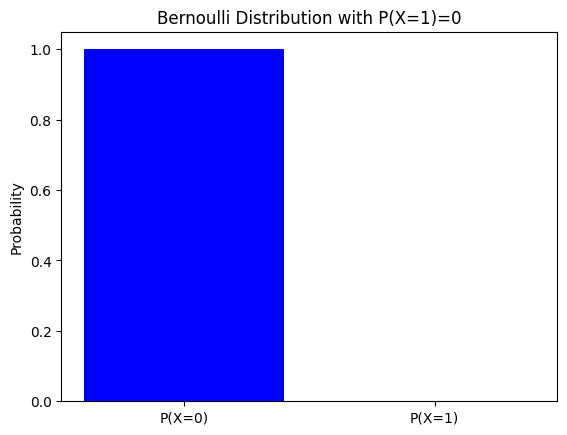
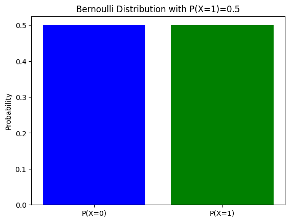
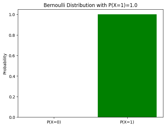
Let’s just write some code to illustrate the Bernoulli distribution:
import matplotlib.pyplot as plt

ps = [0, 0.5, 1.0]  # Showing the probability of P(X=0) and P(X=1) at various values of P(X=1)
P = {}
for p in ps:
    q = 1 - p  # the probability of failure is 1 - the probability of success
    P["X=0"] = p**0*q**1  # P(X=0) = P(x=1)^0 * P(X=0)^(1-0)
    P["X=1"] = p**1*q**0  # P(X=0) = P(x=1)^0 * P(X=0)^(1-0)
    plt.bar(["P(X=0)", "P(X=1)"], [P["X=0"], P["X=1"]], color=['blue', 'green'])
    plt.title(f'Bernoulli Distribution with P(X=1)={p}')
    plt.ylabel('Probability')
    plt.show()
The Binomial distribution: a probability distribution for the number of success#
What we have seen so far:#
To recap what we have seen so far: if we want to know whether a coin is biased, we need to figure out if the probability of head is 0.5:
And according to the Bernoulli formulae:
The Bernoulli distribution describes the rules that control a single coin toss, so to speak. When we throw the coin a single time, we have \(P(X=1)\) chances that it lands on head and \(P(X=0)\) that it lands on tail. Importantly, we don’t know either, which is why we run an experiment. We decided to run an experiment to figure it out. And as we saw before, we had the intuition that for such an experiment, we should be more confident in our results when we increase the number of tosses, because it should be more probable to obtain something close to the true \(P(X=1)\) when we increase the number of throws
The probability distribution of \(P(X=k)\)#
When we are trying to determine what the true probability of success is (\(P(X=1)\)), we ran an experiment in which we toss the coin several times to see how often it lands on head. If the coin is fair (i.e. if \(P(X=1)=0.5\)), then we would expect that the coin is most likely to fall on head half of the time when we toss the coin many times. The number of head we obtain out of a given number of throws also follows a probability distribution. When we toss the coin n times, we have a sample space of size n, because we can out of 10 throws, we can get 1, 2, 3, …, 10 heads. And each of these outcomes is associated with a probability, which depends on the fairness of our coin: if \(P(X=1)=0.5\), then getting 5 head when throwing the coin 10 times is more likely than getting 10 times heads. And in this case again, if we sum the probability of getting 0 head, 1 head, 2 heads… we should get 1. That is because if we throw the coin 10 times, we will most definitely obtain a certain amount of heads: either 0, 10 or everything in between.
We can also write a function that will describe the probability of getting a particular number of successes (i.e. heads) depending on the number of throw and on \(P(X=1)=0.5\), similar to how the Bernoulli distribution describes the probability of getting a particular outcome (1 or 0) depending on \(P(X=1)=0.5\). When you think about it, what we are doing when throwing the coin multiple times, we are actually conducting a series of independent Bernoulli trials. So the probability of getting \(k\) heads out of \(n\) tosses should follow something like this (assuming 5 throws):
That is, the probability of getting 2 heads out of 5 throws is the product of the probability of each event in each trials, so \(P(X=Head) * P(X=Head) * P(X=Tail) * P(X=Tail) * P(X=Tail)\), which gives us:
two times the Bernoulli distribution when \(x=1\) and three times the Bernoulli distribution when \(x=0\). Assuming \(P(X=1)=0.5\) (i.e. our coin is fair):
We can try to make this a bit more general. It is a bit hard to see when we are dealing with a fair coin, because \(P(X=1) = P(X=0)\), but what we have above is basically \(P(X=1)^k * P(X=0)^n-k\) (where k is the number of success). If we imagine an unbalanced coin (\(P(X=1) = 0.3\) for example), this is easy to see:
So a general formulae is the following:
Which is the same as:
This seems like a simple enough formulae: if we know \(P(X=1)\), we can figure out the exact probability of obtaining a certain number of head in our experiment. This is however not entirely accurate, something is missing from our formulae. What we have calculated above is the probability of getting the sequence [head head tail tail tail]. There are several other sequences that yield 2 out of 5 success. To obtain \(P(X=k)\), we need to find all the combinations of heads and tails in which we have 2 heads and three tails. Thankfully, there is an easy formulae to do that:
Which reads n takes k, which is called the binomial coefficient. So if our case, when we want to figure out how many sequences we have that yield 2 heads and 5 tails:
So we have 10 possible combinations. You can try it easily per hand: if you write per hand all the possible sequences, you will also see that there are only 10 that yield 2 heads and three tails. We know that for a given sequence in which we have 2 success, we have the following:
This is true for any sequences in which we have 2 successes, accordingly the probability of getting 2 out of 5 success is:
And so more generally, we have:
With this formulae, we can now compute the probabilty for getting any number of heads out of the number of throws we made, given \(P(X=1)\). But we can also do the reverse: for any values of \(P(X=1)\), we can calculate the probability of our observed number of heads. This formulae is called the binomial distribution.
Relating the binomial distribution to our intuition#
With the binomial distribution, we can validate several of the intuition we had in the previous chapter. For that, we will write a little python function implementing the binomial distribution, thereby illustrating that is nothing terribly complicated!
import math

def binomial_distribution(n, k, p):
    '''
    Calculate the binomial probability P(X = k) for n trials, k successes, and success probability p.
    P(X = k) = \binom{n}{k} p^k (1 - p)^{n - k}
    :param n: Total number of trials
    :param k: Number of successes
    :param p: Probability of success on a single trial
    :return: Binomial probability P(X = k)
    '''
    # Calculate the binomial coefficient (n choose k)
    binom_coeff = math.comb(n, k)  # Calculate n choose k: \binom{n}{k}

    # Calculate the binomial probability using the formula
    probability = binom_coeff * (p ** k) * ((1 - p) ** (n - k))

    return probability
With that simple function, we can obtain the probability for each value of y, while modulating the number of toss we make and the true probability of success.
Logically enough, in the previous chapter, we thought that to figure out whether our coin is biased, we can throw the coin several time. If the coin isn’t biased, then we should be observe head on half of our tosses. This can be simply validated with the formulae above. Let’s look at the probability of each outcomes when we throw the coin 10 times (with \(P(X=1)=0.5\)):
n_throw = 10  # Number of throw
theta = 0.5  # Probability of obtaining head
n_head = range(n_throw+1)  # We want to know the probability of getting 0 heads, 2 heads... up to a 1000 heads out of our 1000 throws


distribution = [binomial_distribution(n_throw,k, theta) for k in n_head]
fig, ax = plt.subplots()
ax.plot([k for k in list(n_head)], distribution)
ax.set_xlabel("k")
ax.set_ylabel("P(X = k)")
ax.set_title("Binomial probability distribution at P(X=1) = 0.5")
plt.close()
Just as we would expect: we are most likely to observe 5 heads than anything else. But none of the other options are exactly 0. Even observing 0 heads or 10 heads don’t have a probability of 0, which means that eventhough they are unlikely to happen, they still might:
print(f"P(X=0) = {binomial_distribution(n_throw, 0, theta)}")
print(f"P(X=10) = {binomial_distribution(n_throw, 10, theta)}")
P(X=0) = 0.0009765625
P(X=10) = 0.0009765625
If we were to repeat the experiment a 10000 times or more, then we might see a couple of times in which we get 0 heads out of 10 throws, so not very likely.
We also had the intuition before that if instead of tossing the coin 10 times to compute \(\hat{P}(X=1)\), we should get more reliable estimates if we toss the coin a 1000 times. That is because we thought the probability of getting \(\hat{P}(X=1)\) that are very different from the true value of the true \({P}(X=1)\) decreases when we increase the number of throws. And we validated this intuition by repeating the same experiment multiple times, as we saw that the values are more constrained in the experiment where we throw the coin a 1000 times compared to when we throw it 1000 times. We can once again prove that this is true by using the binomial formulae. We can compare the probability of obtained \(k/n\) when we throw the coin 10 times or a 1000 times:
theta = 0.5  # Probability of obtaining head

# Prepare figure:
fig, ax = plt.subplots()

# 10 tosses:
n_throw = 10  # Number of throw
distribution_10_throw = [binomial_distribution(n_throw,k, theta) for k in range(n_throw+1)]
ax.plot([k/n_throw for k in list(range(n_throw+1))], distribution_10_throw, label=f"n={n_throw}")

# 20 tosses:
n_throw = 20  # Number of throw
distribution_10_throw = [binomial_distribution(n_throw,k, theta) for k in range(n_throw+1)]
ax.plot([k/n_throw for k in list(range(n_throw+1))], distribution_10_throw, label=f"n={n_throw}")

# 100 tosses:
n_throw = 100  # Number of throw
distribution_10_throw = [binomial_distribution(n_throw,k, theta) for k in range(n_throw+1)]
ax.plot([k/n_throw for k in list(range(n_throw+1))], distribution_10_throw, label=f"n={n_throw}")

# 1000 tosses:
n_throw = 1000  # Number of throw
distribution_10_throw = [binomial_distribution(n_throw,k, theta) for k in range(n_throw+1)]
ax.plot([k/n_throw for k in list(range(n_throw+1))], distribution_10_throw, label=f"n={n_throw}")

ax.set_xlabel("k/n")
ax.set_ylabel("P(X = k)")
ax.set_title("Binomial probability distribution at P(X=1) = 0.5")
plt.legend()
plt.show()
plt.close()
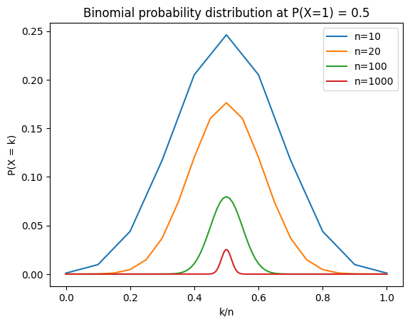
This seems to fit our intuition: the more tosses we do, the more centered on the true value of \(P(X=1)\) the distribution is. Indeed, \(P(X=0.8)\) is largest when \(n=10\) and smallest when \(n=1000\). But you probably also noticed that for any values of \(k/n\), \(P(X=k)\) is lower when we perform more tosses. That is also logical. When we throw the coin a 1000 times, we have a probability for any values between 0 and a 1000, while when we do 10 throws, we have only a value for \(k=1\) to \(k=10\). And because the probability distribution must sum up to 1, it would make sense that the probability of any event is lower when we throw the coin many times. Another way to put it is that when we throw the coin a 1000 times, there are many more possible outcomes (anything from 0 to 1000), so the probability of getting any single value is overall lower compared to when we do only 10 tosses.
The likelihood function: \(P(k|P(X=1))\)#
At this stage, you should understand the concept of probability distribution and how we can build mathematic formulae to describe the probability of any possible outcomes. But at that point, that might seem like abstract mathetmatical concepts and wonder “How does that help us answering whether our coin is biased”? In the graphs just above, I showed the probability associated with each possible outcome in a given experiment. But of course, when you run a given experiment, you don’t really care about all possible outcomes. What you want to know is how much can you trust the outcome of your experiment to infer whether or not your coin is biased. As we said before, what you really want to know is How probable the value of \({P}(X=1)\) is given the data?, so that you can give a principle answer to your colleague.
The binomial distribution is necessary to obtain the probability of the parameter of interest (\({P}(X=1)\)), given the data you have observed. With the binomial distribution, you can not only compute how probable a given value of k is given the number of toss and a given value of \({P}(X=1)\), you can also compute for a single observation how likely that value is under different values of \({P}(X=1)\). This is written as:
The vertical bar means given. So with the binomial distribution you can compute the likelihood of a value of k (i.e. number of success), given a value of \(P(X=1)\) (i.e. probability of head). Say you run an experiment in which you throw the coin 10 times and you obtain 4 heads. You can test what the likelihood of that value is under different \({P}(X=1)\)
import numpy as np
thetas = np.arange(0, 1, 0.01)  # Trying differenet probability of obtaining head
n_throw = 10  # 10 tosses
k_success = 4  # 4 successes

# Prepare figure:
fig, ax = plt.subplots()
k_likelihood = [binomial_distribution(n_throw, k_success, theta) for theta in thetas]
ax.plot(thetas, k_likelihood)
ax.set_xlabel("$P(X=1)$")
ax.set_ylabel("$P(k=4|P(X=1)$")
ax.set_title("$P(k=4)$ given $P(X=1)$")
plt.show()
plt.close()
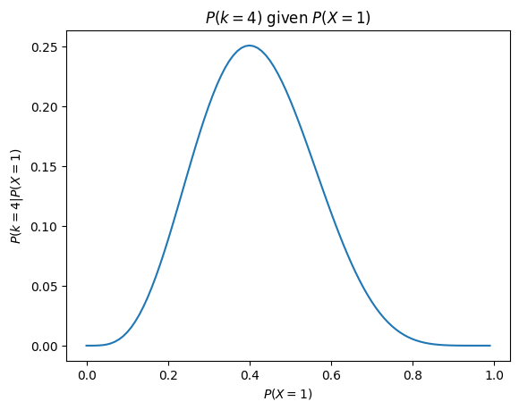
It is crucial to understand what this graph represents. The x axis represents different values for \(P(X=1)\), and the y axis represents the probability of observing 4 out of 10 heads (i.e. \(P(k=4)\)) for each of these values of \(P(X=1)\). Logically, we are most likely to observe 4 heads out of 10 throws if the true value of \(P(X=1)\) is 0.4. This is why the binomial function can be used as the likelihood function: it enables to calculate the likelihood of our observation given any values of \(P(X=1)\).
Our intuition that increasing the number of tosses gives us a more reliable estimate of the true value of \(P(X=1)\) can also be seen here. We can compare the probability of observing 4/10 heads against the probability of observing 400/1000 tosses for different values of \(P(X=1)\):
thetas = np.arange(0, 1, 0.01)  # Trying differenet probability of obtaining head

# Prepare figure:
fig, ax = plt.subplots()
k_likelihood_10 = [binomial_distribution(10, 4, theta) for theta in thetas]
ax.plot(thetas, k_likelihood_10, label="k=4/10")
k_likelihood_1000 = [binomial_distribution(1000, 400, theta) for theta in thetas]
ax.plot(thetas, k_likelihood_1000, label="k=400/1000")
ax.set_xlabel("$P(X=1)$")
ax.set_ylabel("$P(k=4/10|P(X=1)$")
ax.set_title("$P(k=4/10)$ given $P(X=1)$")
plt.legend()
plt.show()
plt.close()
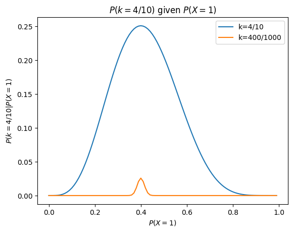
When we throw the coin a 1000 times, many more values of \(P(X=1)\) are very unlikely, which means that uncertainty regarding the true value of \(P(X=1)\) is reduced.
The quantity P(k=4∣P(X=1))P(k=4∣P(X=1)) is directly related to our problem because it tells us how likely our observation is given a specific value of P(X=1)P(X=1). If we find that our observed data is highly unlikely under P(X=1)=0.5P(X=1)=0.5 but much more likely under P(X=1)=0.1P(X=1)=0.1, this suggests that our hypothesis that P(X=1)=0.5P(X=1)=0.5 (i.e., that the coin is fair) might be incorrect. In other words, our confidence in whether the coin is biased depends on how probable our data is under the assumed value of P(X=1)P(X=1).
However, \(P(k=4∣P(X=1))\) is not the quantity we are interested in. We are instead interested in the probability of \(P(X=1)=0.5\), given the data we have observed. In other words, the quantity that we want to calculate is this:
Once again, we can illustrate the difference between \(P(y∣P(X=1))\) and \(P(P(X=1)|y)\) with the same example as before. Say you want to know if it is raining outside, you look out the sky and see that it is cloudy. What you want to know is \(P(P(X=Rain)|y)\) (where y is ‘is cloudy’). This not the same as \(P(y|P(X=Rain))\). The probability of the sky being cloudy when it rains is pretty high, but the probability of rain when the sky is cloudy is not quite as high. Which means we need to add a few additional things to be able to go from \(P(y∣P(X=1))\) to \(P(P(X=1)|y)\).
This is what the Bayes Theorem enables, and this will be the focus of the next chapter