
1 Introduction
The human brain is remarkable in its capacity to learn and perform complicated tasks based on relatively little training and despite limited computational resources. This extraordinary faculty is typically studied in terms of value-based planning, where the task is operationalized as a Markov Decision Process (MDP) to determine which decisions participants should make in order to maximize the reward they obtain throughout the task (REFERENCES). Different reinforcement learning (RL) algorithms can estimate the value associated with each action in any given state in terms of reward maximization, which can be compared to participants behaviour to investigate how optimal their choices are.
However, participants behaviour in complex tasks systematically deviates from optimality (REFERENCES). These deviations are generally thought to reflect the limited processing capabilities of the human brain (REFERENCES). Planning comes at a computational costs, as it typically requires evaluating several alternative futures trajectories in parallel, dependending on actions taken in the future and on the stochasticity of the task, leading to a combinatorial explosion of the outcomes to consider. Accordingly, under computational constraints, one would expect participants to engage in planning to different extents depending on whether it is worth it considering the costs (REFERENCES).
Congruent with this notion of computational rationality, recent studies have suggested that in complex tasks, participants engage in planning to different extent across states of a given task (REFERENCES). It is however unclear on which basis participants decide that certain states require less investment in planning than others (REFERENCES). In this paper, we hypothesized that participants directly exploit the structure of the task to determine the extent to which they should invest in forward planning. Specifically, we hypothesized that participants define a set of simple rules based on each aspect of the task independently such as “Accept high offers more than small ones”, “Accept cheap offers more than expansive ones”… These preferences then get combined when presented with a given state. Prior to reaching a decision, participants evaluate the strength of their composite preference score and the weaker it is, the more they engage in forward planning.
To test this hypothesis, we reanalyzed the data from Ott et al. (2022a) by fitting preferences biases for each factors of the task (offer, energy, current and future costs) and investigating the interaction between the strength of the composite preference score and the decision values to test whether the stronger the preference, the weaker the planning. Our results reveal that participants behaviour are better captured when computing biases scores explicitely based on the structure of the task compared to using more flexible biases models. Importantly, while participants exhibit distinct preferences associated with each aspects of the task, they weight certain aspects more highly than other. Our results suggest that participantss weighting of the task features reflects the relevance of those features in terms of reward maximization. This could either indicate that the dynamics of our task important dyanmics of the environment. Alternatively, this might indicate that participants are able to estimate the relevance of distinct features of the task in their driving influence on the return in the task.
2 Methods
2.1 Participants and experimental design
For this paper, we reused data from a previously published study in which 40 participants (22, mean age=24.4, SD=4.6) took part in a sequential decision making task (Ott et al. (2022a), Ott et al. (2022b)). The study was approved by the Institutional Review Board of the Technische Universität Dresden and conducted in accordance to ethical standards of the Declaration of Helsinki.
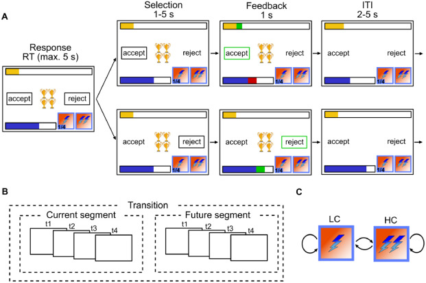
Participants were instructed to gather as many points as possible throughout the task. In each trial, they were presented with offers associated with a reward of 1, 2, 3 or 4 points which they could either accept or reject. To accept an offer, participants had to pay an energy cost of either 1 or 2 energy points. When they rejected the offer, they gained 1 energy point. Participants energy level was capped at 6, so their energy could range from 0 (depleted energy) to 6. Offers varied in each trial following a uniform distribution (equal probability of each offer in each trial). Costs remained fixed for 4 trials segments and participants were informed of the price of the current 4 trials and future 4 trials. The costs of the segment beyond the current horizon was randomly picked such that each costs transitions (from current high or low cost to future high and low cost and vice versa) were equally probable throughout the experiment. If participants accept an offer that they cannot afford (current energy level below current cost), no reward was awarded.
Accordingly, participants had to decide whether to accept or reject an offer based on the current offer and cost ratio. They also had to take into account the impact of their current decision on their future capabilities to accept offers, as systematically accepting offer will deplete energy fast, hindering their capacity to collect more reward. Therefore, maximizing overall return is non trivial in this task and requires complex planning.
2.2 Optimal planning model of choice behaviour
To model optimal behaviour in the task, we operationalized our task as a Markov Decision Process with the following tuples:
\[ MDP = (S, A, P, R) \]
Where \(A\) is the set of possible actions in our task (\(accept=1, reject=0\)), \(P\) is the transitional probability from a given state to all other states (\(P=P_{\forall s \in S}(s'|s, a)\)), and \(R\) is the reward function characterizing the reward participants can obtain in a given state for each action (\(R=R_{\forall s \in S}(s|a)\)). \(S\) represent all possible states in our task, where each state \(s\) consists of a combination of the experimental variables in our task: \(S=E \times O \times CC \times FC \times T\), with energy \(E={0, 1, ..., 6}\), offer \(O={1, 2, 3, 4}\), current segment cost \(CC={1, 2}\), future segment cost \(FC={1, 2}\) and trial \(T={1, 2,..., 13}\). Time steps (i.e. trials) has to be incorporated in the state space to account for the cost being trial dependent. Furthermore, despite knowledge horizon going only until trial 8, we incorporated one segment beyond the known horizon to ensure that future beyond known horizon is considered, otherwise the optimal solution would seek to reach minimal energy level by the end of the 2 segments, which would be detrimental to long term planning.
By extending the time horizon to one trial beyond what is known, we can operationalize the task as an episodic MDP and solve it for the finite horizon of 13 trials. For the trials beyond the known horizon the uncertainty associated with the offer is compounded by the uncertainty related to the costs transition. In trials in the known horizon, the probability of the next state reflects the offer related stochasticity while the rest is deterministic, based on participants actions and structural constraints of our task (see Ott et al. (2022a) for more details and here).
We applied backward induction to the MDP to compute value associated with each state and the value associated with each action in each state (V and Q functions respectively, see Sutton et al. (1998)). If participants behave optimally, their behaviour should reflect a softmax function over the value associated with each action in a given state ([REFERENCE])e, which in the case of a binary decision problem simplifies to the logit function (see Lepauvre and Kiebel (2026) for proof):
\[ \begin{align} P(a=1) &= \frac{1}{1+e^{DV}} \\ where\ DV &= Q(s, a=1) - Q(s, a=0) \end{align} \]
2.3 Modelling participants preferences
In addition to the planning component, it was previously observed that participants behaviour differs significantly depending on the offer. Specifically, it was observed that participants respond significantly faster yet less optimally when offers were either high or low (o=1 and o=4) compared to intermediate offers (o=2 and o=4). This was interpreted as indication that participants consider that the task consists of two separate offer-based contexts, and inferred that the intermediate offer context required more careful planning than the extreme offer context.
In this work, we aimed to investigate whether instead of a binary contextualization of the task, participants behaviour reflects a weighted combination of a planning component with preferences reflecting the structure of the task. Specifically, we hypothesized that the data can be explained by a weighted combination of preferences associated with each levels of each factors of the state space. This idea can be formalized using the following model:
\[ \begin{align*} P(a=1) &= \frac{1}{1+e^{\eta}} \\ where\ \eta &= \beta_{plan} \times Q(s, a=1) - Q(s, a=0) + \mathbf{X_{pref}}\mathbf{\beta} \end{align*} \]
Where \(\mathbf{X_{pref}}\) is a \([M \times N]\) (M=measurements, N=experimental levels) matrix dummy coding each factors of the experimental design (energy, offer, current and future costs), and the \(\mathbf{\beta}\) is a vector of weights estimated for each levels of each factors of the experimental design. In other words, in addition to the planning component, we estimated weights associated with each experimental factors to compute a compound preference score. Beyond the mere combination of planning and preferences, we sought to investigate whether participants behaviour reflects an interaction between the two, whereby if participants rely more or less on planning depending on whether they have weak or strong preferences in a particular state (preferences scores closer or further away from 0). This required us to estimate the latent preference score component from the data and test for possible interaction with the planning component. However, as our interaction relate not to the raw preference scores but to their strength, we transformed the preference score to entropy. In other words:
\[ \begin{align*} P(a=1) &= \frac{1}{1+e^{\eta}} \\ where\ \eta_{preference} &= \beta_{plan} \times DV + Preference + \beta_{Interaction}(H(Preference) \times DV) \\ with\ Preference &= \mathbf{X_{pref}}\mathbf{\beta_{pref}} \end{align*} \]
In addition to this model, we fitted both the planning model and hybrid model from Ott and colleagues (Ott et al. (2022a)). Specifically:
\[ \begin{align*} \eta_{planning} =& \beta{plan} \times DV + \\ &\beta_{basic}\mathbf{I}_{basic} + \beta_{maxE}\mathbf{I}_{maxE} + \\ &\beta_{minE_{LC}}\mathbf{I}_{minE_{LC}} + \beta_{minE_{HC}}\mathbf{I}_{minE_{HC}} \end{align*} \]
\[ \begin{align*} \eta_{hybrid} =& \beta{plan23} \times DV_{23} + \beta{plan14} \times DV_{14} + \\ &\beta_{O1}\mathbf{I}_{O1} + \beta_{O2}\mathbf{I}_{O2} + \beta_{O3}\mathbf{I}_{O3} + \beta_{O4}\mathbf{I}_{O4} + \\ &\beta_{basic}\mathbf{I}_{basic} + \beta_{maxE}\mathbf{I}_{maxE} + \\ &\beta_{minE_{LC}}\mathbf{I}_{minE_{LC}} + \beta_{minE_{HC}}\mathbf{I}_{minE_{HC}} \end{align*} \]
Where \(\mathbf{I}\) indicate dummy regressor encoding specific experimental conditions: \(\mathbf{I}_{basic}\) encode trials where energy is sufficient to accept the offer and inferior to 6, \(\mathbf{I}_{maxE}\) encodes trials where energy is equal to 6, \(\mathbf{I}_{minE_{LC}}\) for trials where energy is too low to accept the offer when cost is low, \(\mathbf{I}_{minE_{HC}}\) for trials where energy is too low to accept the offer when cost is high, \(\mathbf{I}_{minE_{O1-4}}\) for trials with offer 1-4 where energy is sufficient to accept.
2.4 Model fitting and comparison
The model described above were fitted on participants responses data as Bayesian hierarchical logistic regressions using PYMC (Abril-Pla et al. (2023)) and Bambi (Capretto et al. (2022)), (see Lepauvre and Kiebel (2026) for the exact models). We excluded trials where participants reaction time (RT) exceeded the response window (5s) or didn’t provide a response. Across models, the following parameters were left to vary across participants (i.e. random slope): \(\beta_{plan},\ \beta_{plan23},\ \beta_{plan14},\ \beta_{pref},\ \beta_{Interaction},\ \beta_{basic},\ \beta_{O1},\ \beta_{O1},\ \beta_{O2},\ \beta_{O3},\ \beta_{O4}\), while the rest were fixed across participants. For all parameters, we used weakly informative hyperprior distributions \(\mu \sim \mathcal{N}(0, 2)\) and \(\sigma \sim Halfnormal(0, 2)\). All models were fitted using 4 chains of 2000 sample each (1000 warmups), resulting in 16000 samples in total.
We used Pareto-smoothed importance sampling to approximate leave one out cross validation (PSIS-LOO, Vehtari et al. (2017)) to estimate the expected log pointwise predictive density (elpd) which we used to compare the fit of these different models.
Furthermore, we perform model comparison within each single subject to estimate the robustness of the winning model in our population sample, but computing the sum of the pointwise predictive accuracy for each participant and model, yielding a score for each participant and model.
2.5 Reaction times analysis
Following the observation that modelling choice behaviour as a function of preferences, decisions values and the interaction between the two fitted the data best, we hypothesized that the degree to which participants engage in effortful foward planning in a given state depends on the strength of their preferences. If that is the case, this should be reflected in participants reaction time (RT), such that the stronger their preferences (i.e. the lower their preferences entropy), the lower their RT. Importantly, as it was previously observed that participants RT increases when decision values are close to 0, which was interepreted as evidence that participants are able to reach a decision quicker when the value asssociated with one decision is much higher than that associated with any other decisions Ott et al. (2022a). In this paper, they further observed that participant RT depended more on decision values in intermediate offers (2 and 3) compared to extreme ones (1 and 4), which they interpreted as evidence that participants consider these offer groups as separate contexts, with the latter requiring more forward planning than the former.
Here, we predicted that the driving factors of reaction time was not simply offer groups but rather the strength of participants state-specific preferences. In other words, it is possible that the reason participants treat intermediate and extreme offers differently is because of different overall preferences associated with states presenting such offer. By fitting preferences directly in the previous model we can investigate with a greater granularity how they shape reaction time when combined with decision values. We modelled the log of reaction time using the following model:
\[ log(RT) = \beta_{plan} * DV + \beta_{pref} * H(preferences) + \beta_{interaction} * (DV : H(preferences)) \]
Where \(preferences\) is the preference score fitted from the preference choice model above, and \(H\) stands for the binomial entropy function. We compared this model to Ott et al. (2022a) RT model to test whether the use of preference fits the data better than a dichotomous distinction between intermediate and extreme offers, which would indicate that participants consider the strength of their preferences to determine how much they should invest in planning and that the observation of the distinction between intermediate and extreme offers is a byproduct thereof.
2.6 Task structure importance
Our choice and reaction time results replicate and extend on Ott et al. (2022a) findings. We indeed observed that deviation from optimal value based decisions depends strongly on offer as well as on energy. Our results further indicates that these deviations reflect composite preferences derived from the structure of the task. Our results also suggest that not all dimensions of the task are weighted equally in participants preferences. To further quantify the importance associated with each factor of the task (offer, energy, current and future cost), we performed a model comparison in which we remove the preferences associated with each factor of our task (i.e. removing all regressors associated with offers, energy, current and future costs one at a time) to identify how much of the fit is explained by each.
In addition, we computed the expected cummulative return when the optimal policy is derived from a reduced MDP of the task, in which we selectively remove each factor of the task. Specifically, we created reduced MDPs in which we averaged the transition probability and reward associated with all levels of each factor to investigate what the optimal return would be for a planner that selectively ignores a given aspect of the task. We then computed the optimal policy on this reduced MDP, and applied this optimal policy from the reduced MDP back to the full MDP. This analysis is meant to investigate whether participants’ weighting of the factors in their preferences reflects the dominant structures in the task driving the return.
3 Results
3.1 Choice behaviour
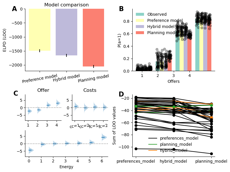
In line with Ott et al. (2022a), we observe that a model taking only planning component into account does not perform as well compared to taking state specific biases into account. Importantly, the preference model was found to significantly outperform the hybrid model, indicating that participants biases do reflect the structure of the task (see Figure 2 A). When investigating the fitted preferences parameters, we observe that participants exhibit strong offer based preferences, such that they tend to reject low offers (1 and 2) more than dictated by the decision values and accept larger offers more than they should (see Figure 2 B), and this bias is more extreme for more extreme offers (1 and 4) than intermediate ones (2 and 3). For costs, the estimated preference parameters all significantly overlap 0, indicating that participants do not show strong biases away from optimal decision based on these factoors. Participants show strong preferences when energy is at 0 (systematically reject) and at 6 (almost systematically accept regardless of any other conditions, see below). In intermediate values, participants show a midly incremental preference, such that they have a tendency to reject offers slightly more than they should when energy is low, but are increasingly likely to accept when energy increases.
The results broadly replicate Ott’s findings, as they show that participants treat high and low offers quite differently, with a further modulatory effect of energy, reflecting the energy specific parameters from Ott’s model (\(\beta_{basic}, \beta_{maxE}, \beta_{minE_LC}, \beta_{minE_HC}\)).
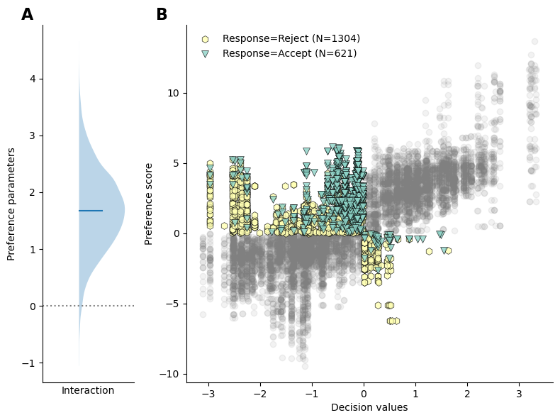
Importantly, our model revealed a positive interaction between preferences entropy and decision values (\(\beta\)=1.74, CI=[0.38, 3.07], see Figure 3 A), indicating that participants weight decision values higher when their preferences are weak and vice versa. Figure 3 B depicts participants responses as a function of decision values and fitted preferences, the grey dots represent trials in which both the preferences and decision values were matched (either both positive or both negative), while colored markers indicate trials in which preferences and decision values were misaligned, color coded by participants responses (green triangles: accept, yellow hexagon: reject). Importantly, rejected trials in the upper left quadrant of the figure indicate that participans responses follows the decision values but goes against the preference, while accepting indicates that participants actions follows the preference to the detriment of the decision values, and vice versa in the bottom right quadrant.
As we can see from Figure 3 B, when preferences are positive and decision values negative (top left quadrant), participants tend to accept the offer when the decision values are close to zero, reflected in the green triangles data points clustering towards 0 on the x axis. In contrast, participants tend to reject the reward more often when the decision values grow more negative, illustrated by the increased number of yellow dots on the left extremities of the top left quadrant. Similarly, when decision values are positive and preferences negative (bottom right quadrant), participants tend to reject the offer more often when the decision values are small, and accept the offer more often when the decision values grow larger (though the number of samples is much lower in this quadrant). These observations reflect the positive interaction between preferences entropy and decision values, indicating that participants rely more on preferences when decision values are close to 0 and vice versa.
3.2 Reaction times
In a task as large as ours (448 single states), computing the exact value associated with each state is costly. In comparison, preferences, are presumably readily available to the participants, or require minimal computation. The interaction between the two observed at the responses levels suggests that participant control the planning demands depending on the strength of their preferences, such that if their preferences are really strong in a particular state, they would dedicate less effort to forward planning. Indeed, Ott et al. (2022a) observed that RT grew significantly more rapidly in intermediate offers as a function of the magnitude of decision values compared to extreme offers, indicating that participants dedicate less cognitive effort to the extreme offers, which they interpret as evidence that these constitute two distinct contexts.
Importantly, these differences in RT patterns observed between intermediate and extreme offers might in fact be driven by differences in overall preference strength between both these conditions rather than these conditions being treated as separate contexts. In other words, we hypothesized that participants investement in forward planning depends on the strength of their preferences, and we therefore predicted that reaction time (indexing forward planning) should reflect the strength of the decision values and of their preferences as well as the interaction between the two rather than an interaction between decision values and intermediate offers (as was found in Ott et al. (2022a)). Specifically, we expect a positive interaction between conflict (i.e. negative amplitude of the decision values) and the preference entropy, indicating that participants reaction time increase more rapidly as a function of decision values when preferences are weak (i.e. entropy is high).
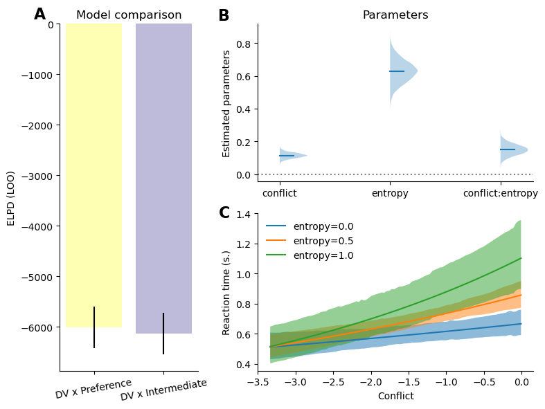
In line with this prediction, modelling reaction time as a function of preferences and conflict as well as the interaction between the two performs better than Ott et al. (2022a) original model (see Figure 4 A). We observed a positive interaction effect between preferences entropy and conflict (see Figure 4 B), indicating that participants reaction time is more strongly dependent on decision values when preferences are weak (i.e. high preference entropy, see Figure 4 C). Combined with the response choice models, these results reveal that the participants decreased accuracy and reaction time in extreme offers compared to intermediate offers reflects participants stronger preferences in these conditions.
3.3 Variables weighting
We observed that both response selection and reaction time reflect value-based combined with preferences and that these preferences themselves reflect the structure of the task. Specifically, our results suggest that participants have preferences related to each factors of the task that then get combined to generate a composite preference score in a given state. Importantly, not all features of the task are weighted equally. Indeed, we can see in Figure 2 C that the parameters associated with offers and energy weight higher than cost in the preference. To further characterize these differences, we compared models in which the preferences associated with each factor of our task were removed one at a time.
Figure 5 displays the difference in fit between the full preference model against models in which the preferences related to each experimental factor was removed, larger values indicate that the factor account for a more important proportion of the full model’s fit. These results indicate that energy followed by offer have a much larger impact on participants final responses, whereas costs related preferences have a small impact on the overall fit.
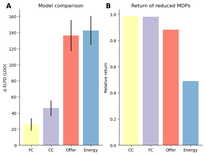
This differential weighting of experimental factors in participants preferences might reflect the fact that humans are generally biased to attend to certain features (such as reward and energy) over others, due to their overall relevance in the environment. Alternatively, these may reflect that based on the structure of our task, certain features might be more relevant than others to maximize rewards, such that when ignoring more relevant dimensions of the task when planning leads to larger reward loss than other. If that is the case, an agent with limited processing capabilities should attend to this features more, which might be what the differential weighting of participants’ preferences reflect.
To provide substantive evidence for the latter claim, we computed the expected return from simplified representations of the task in which each experimental factor is omitted one at a time, to quantify the loss in reward associated with ignoring it. The results are shown in Figure 5 B. We observe that order of the factors in terms of their relevance for returns is reminescent of participants’s weighting of those factors in their preferences. Indeed, both current and future costs have relatively low impact on the overall return, while offer and more critically energy have a larger impact, which reflects preferences weighting. While this does not constitute decisive evidence, these results suggests that participants preferences might not only reflect bias based on previous experience in their environment, but might also be adapted to the structure of the task.
4 Discussion
High level summary of results interpretation
Discuss how the results relate to the notion of computational rationality and policy compression In policy compression framework, planning is complemented by the marginal action probability which is taken to constitute a prior over action. Our use of preferences constitutes an extension to it. Instead of considering marginal probability across states, our preferences define action probability based on the structure of the task, informing the default policy of subjects beyond what is done in traditional policy compression. Or put differently, in policy compression, assuming that participants are under too much pressure to rely on planning, participants should rely on state independent action prior, which is very restrictive and probably not adaptive. It is likely that participants rely on more information to make adaptive decisions even when planning is limited. Our Preferences offer a solution to this
Discuss how the results relate to Sarah’s model (2024 PLoS CB paper) and the idea of Certainty-based stopping criterion
Discuss how the results relate to the traditional distinction between habits and goal directed. Preferences might reflect the habit process, and our results might indicate that both modules are at play, just that planning kicks in only if habits are weak, also in line with Sarah’s work on balancing habits and goal directed behaviour paper from 2021
Future experiment: have participants conduct several versions of the same task in which different features of the task drive the return (i.e. make cost more relevant for example) and see how that influences the preferences weighting.
A limitation of the present work is we assume that preferences are fixed, thought they are likely to be dynamically updated throughout the task. Future work should aim to characterize preferences update mechanisms, by dynamically updating both the reward and transitional probabilty structure of the task, either in a gradually or chunk-wise (i.e. having separate experimental blocks with different task structures).
5 References
Abril-Pla, Oriol, Virgile Andreani, Colin Carroll, et al. 2023. “PyMC: A Modern, and Comprehensive Probabilistic Programming Framework in Python.” PeerJ Computer Science 9: e1516.
Capretto, Tomás, Camen Piho, Ravin Kumar, Jacob Westfall, Tal Yarkoni, and Osvaldo A Martin. 2022. “Bambi: A Simple Interface for Fitting Bayesian Linear Models in Python.” Journal of Statistical Software 103 (15): 1–29. https://doi.org/10.18637/jss.v103.i15.
Lepauvre, Alex, and Stefan J Kiebel. 2026. Preferences for Forward Planning in Human Decision-Making-CODE. V. 0.1. Zenodo, released. https://github.com/AlexLepauvre/state_abstraction_paper.
Ott, Florian, Eric Legler, and Stefan J Kiebel. 2022a. “Forward Planning Driven by Context-Dependant Conflict Processing in Anterior Cingulate Cortex.” NeuroImage 256: 119222. https://doi.org/10.1016/j.neuroimage.2022.119222.
Ott, Florian, Eric Legler, and Stefan J Kiebel. 2022b. Forward Planning Driven by Context-Dependent Conflict Processing in Anterior Cingulate Cortex - Analysis Code and Datasets. V. 1.2. Zenodo, released. https://doi.org/10.5281/zenodo.6328296.
Sutton, Richard S, Andrew G Barto, et al. 1998. Reinforcement Learning: An Introduction. Vol. 1. MIT press Cambridge.
Vehtari, Aki, Andrew Gelman, and Jonah Gabry. 2017. “Practical Bayesian Model Evaluation Using Leave-One-Out Cross-Validation and WAIC.” Statistics and Computing 27 (5): 1413–32.